Geodesic Geometrics
Series index: Part I, Part II, Part III (this post)
Part II established that recursive midpoint, one-pass
After quantifying the discrepancies, I need to reveal uncomfortable truths about geometry to budget unavoidable distortion. But first, a side quest.
Side quest: why icosahedra? §
Before comparing algorithms, I’ll detour to the question, “to approximate a sphere with a triangle mesh, why start subdivision with an icosahedron as our root solid, when—to quote the BBC—other Platonic solids are available*?”
A simple answer is, “it has the most faces.” More faces mean that each face soaks up less of the total curvature of the sphere, making it a better approximation of the patch of spherical surface it represents, leading to less distortion resulting from projecting a flat triangle onto a curved sphere.
However, that’s not the most convincing argument since we can produce subdivision algorithms almost as quickly as they can generate new faces. So to really answer the question, I have to think about curvature.
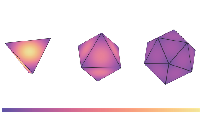
First, the curvature of a plane: zero. Sum of angles around a point on a plane: 360º. So, if we want to join regular (equilateral) triangles—whose interior angles include 60º—around that point, we can fit exactly six of them, creating a 6-triangle vertex†. Those six triangles comprise a regular hexagon, which as you might know can tile the plane without gaps or overlaps.

To wrap fewer regular triangles around a point—say, only three—then the triangles must rise out of the plane until their edges join, closing the gap left by the missing three corners‡. Those corners represent a half-circle worth of missing angle that must be made up by the folding, a rather literally-named angular defect§.
Finally, let’s replicate that construction of “three triangles around a point” for each of the new vertices we just created, and so on, until we have a full sphere’s worth of curvature. We just built the regular tetrahedron, one of the five Platonic solids.
How about other numbers of equilateral triangles we can arrange around a point (degenerate cases in italics)?
| Triangles (degen) | Angular defect | Explanation |
|---|---|---|
| 0 | “360º” | A point with… no triangles |
| 1 | “300º” | Just a triangle, not a polyhedron |
| 2 | “240º” | Degenerate in Euclidean space and indistinguishable¶ from a triangle: a dihedron |
| 3 | 180º | Tetrahedron |
| 4 | 120º | Octahedron |
| 5 | 60º | Icosahedron |
| 6 | 0º | Planar triangular tiling |
| 7 | -60º | Non-convex |
This table suggests that at least three regular triangles are needed to form a vertex that encloses curvature and form a regular convex polyhedron. But, no more than five equilateral triangles fit around a convex vertex, else they include so much angle that they form a flat plane or even a non-convex surface (think “saddle point”).
What about other regular polyhedra? The other two Platonic solids, the cube (“regular hexahedron”) and dodecahedron, are made of squares and pentagons♠, respectively, so we can skip those. As for the remaining 43 regular polyhedra…
… wait, what?
Side side quest quest: the 48 regular polyhedra §
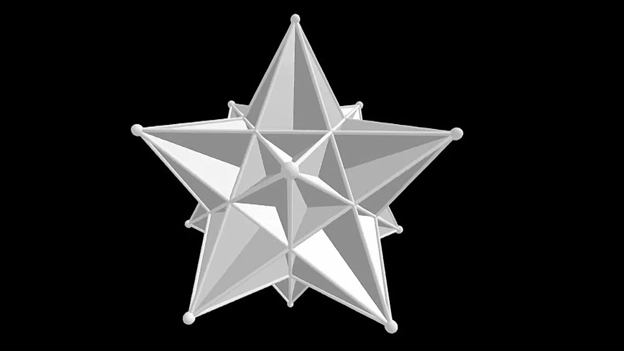
Alright, it turns out that we normies aren’t being specific enough with our search for solids for subdivision, if we only specified “regular polyhedra.” We also should stipulate that we want them to be convex, and in fact comprise planar faces that don’t intersect each other and aren’t tilings, to appropriately rule out the Petrial small stellated dodecahedron♥.
I highly suggest a delightfully destabilizing trip through these rejected candidates.
Back to icosahedra §
So if polyhedra with regular triangular faces are the constraint, the faces’ least curved arrangement (before they tile into a plane) puts five around each vertex, forming a regular icosahedron, which—as a result—has the most faces of such polyhedra. “Most faces” is a good criterion for “best root solid” because it provides the best approximation of a sphere and requires less subdivision, but do root triangle count and shape affect resulting polysphere quality?
After all, if—and this is the tragically-sized if from Part I—we can subdivide equilateral triangles into arbitrarily many smaller equilateral triangles, does it really matter if we start with a tetrahedron or an icosahedron?
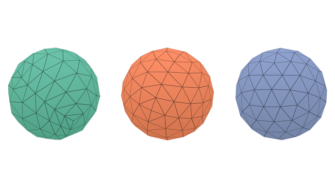
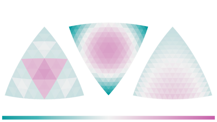
Clearly, it does matter. The “tetrasphere” (left) looks like a mutant Brassica while the “octasphere” (middle) looks like it has three pairs of criss-crossing “poles.” They clearly contradict our hypothesis about the properties of subdivided equilateral triangles because they absolutely do not look like they’re made of equilateral triangles. Does that mean that the icosphere (right)—“icosasphere?”—is made of faces that aren’t perfect congruent equilateral triangles?
What does “perfect” mean? §
At the start of this project, I had a practical definition of “perfect” for this specific mesh-building problem: all faces stay congruent and equilateral after projection. So in metric form, that means:
- Area uniformity: coefficient of variation (CV) over triangle areas♦
- Angle regularity: mean absolute deviation from 60° over corner angles♣
- Bonus readout: ratio of the areas of the largest and smallest triangles, which establishes the distribution of outliers, not only RMS spread
Now perfection can be quantified, namely, as when the main metrics fall to zero:
| Metric | Lower is better | Intuition |
|---|---|---|
| Area CV | Yes | Are triangles similarly sized? |
| Angle mean deviation (from 60°) | Yes | Are triangles similarly shaped? |
| Area max ÷ min | Yes (best = 1) | How severe are outliers? |
Test setup & results §
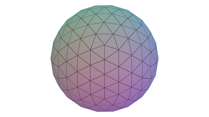
We take a single wedge of the root icosahedron and subdivide it to 256 triangles using each method. This compares the methods at a fixed triangle count that both exponential and quadratic subdivision can achieve. It’s high enough to provide decent statistical resolution for the metrics, but low enough that a shader visualization of each face’s distortion remains intelligible.
Measurements §
| Method | Area CV | Mean deviation from 60° | Area max / min |
|---|---|---|---|
| Recursive midpoint ( | 8.6% | 7.1º | 1.30 |
| One-pass | 13.3% | 3.2º | 1.86 |
| Direct slerp ( | 4.6% | 6.4º | 1.19 |
Observations §
- To my complete surprise, direct slerp beats recursive midpoint for all three. I thought of recursive midpoint as the gold standard.
- One-pass
Where is the distortion? §
The aggregate metrics are useful, but to understand where the distortion lives, I built a visualization to show the spatial structure. It shades each triangle according to its local distortion, then plots the results for each method side by side to compare.
For both metric modes, the color shows signed divergence from the ideal; left half of the range indicates deflation from each wedge’s mean or deficiency from 60º, while the right half indicates inflation or excess angle. In both modes, the range is scaled to the maximum distortion observed across all three wedges, so the same color in different wedges corresponds to the same amount of distortion.
Observations §
- Each time we perform a Loop split in recursive midpoint, the center triangle of the four new triangles inflates while the surrounding triangles deflate, a pattern that repeats recursively. This produces a
triforcefractal-like pattern with some strong, sharp edges between inflation and deflation caused by the first pass that’s preserved at higher recursion generations. - One-pass
- In angle mode, we can see that the corners of the wedges have a strong expansion of angle.
- In angle mode, most triangles have one broadened corner and two narrowed corners, not the other way around, creating squat (not tall) practically-isosceles triangles. There are many pairs of triangles whose shared edge has sharpened corners on both sides, forming little diamonds.
- Direct slerp has a directional asymmetry, more visible in area mode: modest contraction along the first two slerp edges and slight expansion toward the row-aligned third edge.
The first one actually seems like a genuine issue. Imagine if you textured the sphere with a circle that intersected one of the very inflated center triangles and one of the very deflated edge triangles: the circle would look like a teardrop¤. The smooth gradation of distortion from the center to the edge is actually a feature of the one-pass
That ties into the last observation, which is a bit unsettling: direct slerp’s distortion field is not dihedral symmetric. I’m not sure why this is happening, but it means that it’s possible to stitch the wedges together in a way that produces discontinuities between them (and it’s possible to avoid this).
What’s going on? §
OK, neither of the promising methods is perfect. Instead, it seems like there are some unavoidable tradeoffs between area and angle distortion. Why?
Intuition: the Platonic ceiling §
The side quest was secretly Tutorial Island. Regular triangular faces are the constraint and an icosahedron already packs the most such faces on a convex regular polyhedron. That’s the ceiling. We can’t keep adding triangles while preserving that exact regular-triangle perfection everywhere.
Intuition: adjacency and curvature §
Besides, think about the connectivity of the new triangles added; all new vertices are 6-triangle. Six 60º corners (“0 angular defect”) around a point is a plane, but we want positive curvature.
So we’re trying to add more triangles to a peak-triangle Platonic solid and those new triangles don’t even want to be on a curved surface. Something has to give.
Unintuitive: spherical triangles scale funny §
Look at what actually happens to the corners of the wedge as it’s being subdivided, like the animation from Part I.
As visible in the distortion figure’s angle mode and in the subdivision animation, the corners of the root solid widen in angle with each round of subdivision. It’s no coincidence that this is happening as the wedge is becoming more spherical; after all, the whole point of these methods is to approximate and converge to a perfect sphere (regardless of unevenly-distributed triangle areas). This behavior holds for all three methods, because it’s not a bug, but a property of spherical geometry.
A high school geometry fact: the angles of a triangle sum to 180º. Well… that may be true for planar triangles, but on the surface of a sphere, a triangle (a spherical triangle) obeys different rules. The sum of its angles can range from 180º to 540º, depending on the area of the triangle.
The side quest comes in handy again. A closely-related concept to angular defect measured with a triangle wrapped around a polyhedron’s vertex, the spherical excess of a spherical triangle is the amount by which the sum of its angles exceeds 180º.
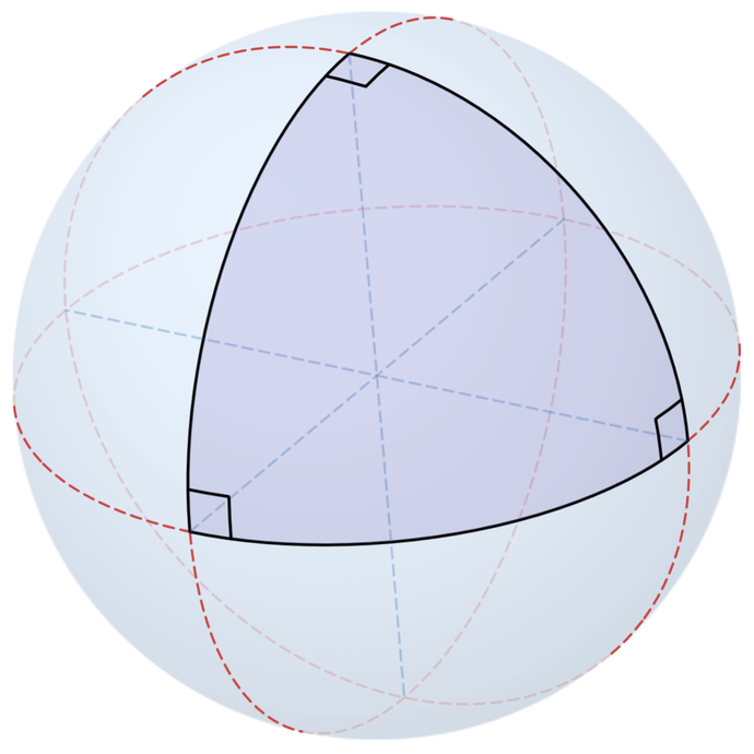
Wikimedia Commons, User: Jacobolus, CC BY-SA 4.0
In fact, the spherical excess
By the way, this surface area of a shape projected on a unit sphere is also known as the solid angle subtended by that shape, out of a total of
For a regular icosahedron (which has 20 faces) projected onto the unit sphere, each spherical triangular face has area
Yup. As the wedge becomes more spherical, the corner angle must widen from 60º to 72º. That explains the corner inflation in the distortion figure’s angle mode for all three subdivision methods. However…
Scaling spherical triangles §
Quarter that icosahedron face by surface area—assuming we can do that perfectly—to arrive at
Interesting. Unlike the planar case, where subdividing a triangle into smaller triangles of equal shape simply scales down without changing the angles, subdividing a spherical triangle into four smaller triangles of equal area produces triangles with narrower angles. This makes sense; as the triangle gets smaller, it basically becomes more planar, so it tends towards 60º corners.
But imagine trying to fit one of those smaller triangles into the original corner of the wedge. How is this quarter-face triangle supposed to fit in the 72º corner of the original face if it only has 63º corners††?
That drives a new pair of nails in the coffin of the big if from Part I. Not only are equilateral planar triangles unable to fill the spherical triangle projected from an icosahedron’s face—because the angles don’t match—spherical triangles can’t even subdivide into smaller spherical triangles of the same shape—because the angles don’t match.
Mapmakers’ dilemma (maybe trilemma?) §
In the back of my mind, I always figured that this was either a solved problem (remain blissfully unaware of midpoint subdivision’s distortion and move on) or—more likely and now confirmed—an unsolvable problem with well-studied tradeoffs. The field in which those tradeoffs are studied? Cartography.
After all, mapmakers have been trying to solve this exact problem for millenia, just on a bigger scale. They’re trying to flatten a sphere onto a plane, not simply a patch of a sphere onto a triangle. It’s the same problem, however. The curved surface can’t be flattened without distortion. I need to draw from cartographers their sophisticated analysis of the tradeoffs and their rich library of map projections that distribute distortion in different ways for different uses.
So, let’s segue from abstract geometry to the art of Earth measurement, which you might call “geo metrics.” That is, let’s change the topic from geodesic geometry to, if you will, geo-metric geodesy.
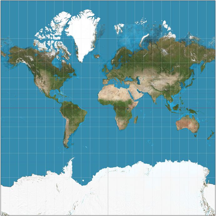
Wikimedia Commons, User: Strebe, CC BY-SA 4.0
The most (in)famous tradeoff is that a 2D map, even of an idealized spherical Earth, can’t preserve both scale and shape‡‡ (and often preserves neither!).
The deservedly much-maligned Mercator projection—with its inflated Greenland and hyperbolic vertical extents that obscure poles—is actually the result of making this tradeoff; it’s in fact the only single-split seam (uninterrupted) projection that preserves angle (conformal) and also has straight longitude lines (meridians). These properties were intended for navigation in the era before GPS. And now, in the era of cloud mapping software, its modern descendant, Web Mercator, is still considered the most practical choice for the way most people and software interact with maps: zoomed in, north-up, inside Google software that abstracts Earth as a square, and expecting street shapes to match the local geometry regardless of being in Stockholm or Guatemala City.
Let me interrupt you §
However, there is another lever besides “area vs angle”: interruptions. When the globe is cut into more pieces, each piece can carry less distortion of both kinds, at the cost of “point to point” continuity when laid out flat. This is the “flatten an orange peel” analogy; you can’t do it without tearing the peel, so… tear it.
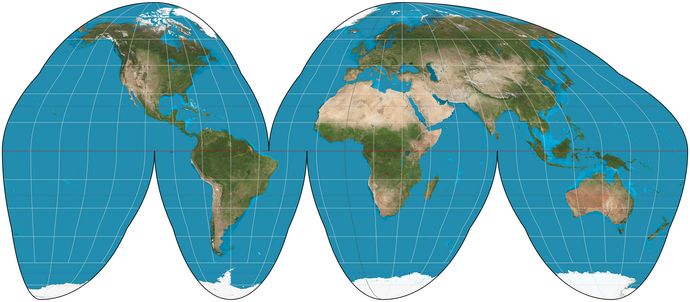
Wikimedia Commons, User: Strebe, CC BY-SA 4.0
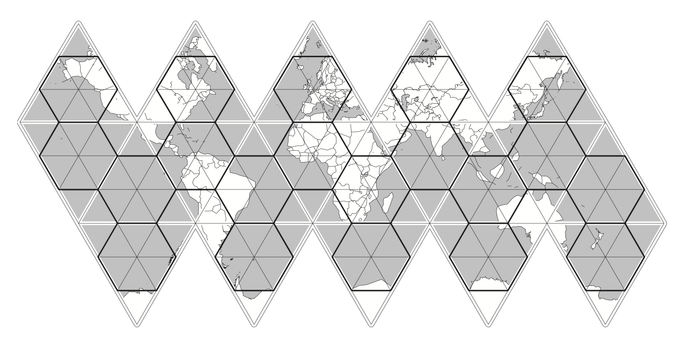
Well, what else can be cut into pieces? Polyhedra, of course. Specifically, some can be cut into nets, 2D layouts of their faces that can be folded back into 3D solids. As for which polyhedron, the icosahedron is again a good choice that evenly distributes distortion over as many equilateral triangle faces as possible. Naturally, good ol’ Bucky Fuller came up with the Dymaxion projection§§.
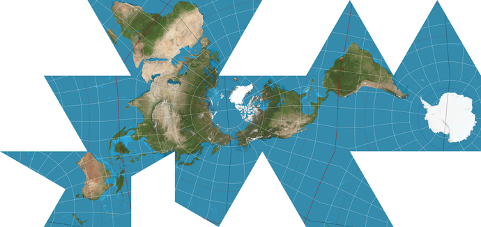
Wikimedia Commons, User: Justin Kunimune, CC BY-SA 4.0
If cartographers can cut a sphere into 20 triangular faces to reduce distortion in each face, then do they have methods to further cut the sphere into even more, smaller faces that each have even less distortion?
Geodesic geodesy §
To put the cartographic perspective on our problem, let me go over the parallels between our solutions and map projections.
Point distortion §
First, the distortion introduced by Mercator is fundamentally the same as that introduced by one-pass
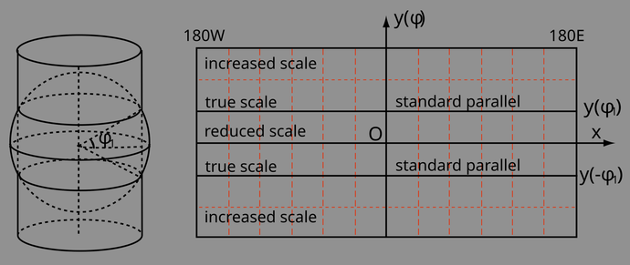
Wikimedia Commons, User: Peter Mercator, Public Domain
A cross-section along a meridian looks just like the lerp-slerp diagram, only instead of projecting a chord to its arc, it projects an arc to its tangent line. The Mercator area distortion pattern along a meridian is exactly the inverse of the edge inflation distortion pattern caused by the one-pass
The tangent projection can be generalized in another way. A gnomonic projection skips the “project to, then unwrap a tangent cylinder” step and projects directly from the sphere’s center to a plane, which is only tangent to the sphere at a single point.
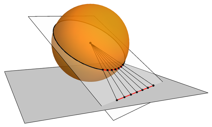
Wikimedia Commons, User: Marozols, CC BY-SA 3.0
Its distortion pattern is an even better analog to our distortion map, because its projection incurs this error in every direction, not just along a meridian. If the Mercator projection’s distortion is like the inverse of the one-pass
Subdivision §
Second, geo dudes do want to solve our subdivision problem, because there’s more to geodesy than making maps. Subdividing the globe into smaller regular regions is a useful step for geospatial pipelines. For that, the lat-long grid, or graticule, doesn’t cut it. In much the same way that UV spheres are limiting for graphics, the graticule doesn’t uniformly distribute geospatial location over its coordinates♠♠.
Maybe unsurprisingly, the icosahedron is a popular choice for creating such discrete global grid systems (DGGSs). For reasons reminiscent of why we chose the icosahedron as our root solid, the most popular shape for grid cells of DGGSs are hexagons (… mostly). They let grid users treat cells like the best possible approximations of smooth, round patches of land that fit together tightly. Uniquely, tiled hexagonal cells have an advantage: any two neighboring cells share an edge. Meanwhile, recursive subdivision is a feature for such systems, as “number of rounds of subdivision” provides a convenient basis for hierarchical indexing and levels of grid resolution.
McCollum et al. 2008. A discrete global grid of photointerpretation.
Then is it possible to go from an icosahedron to a grid of equal-sized regular hexagons tiled over the sphere? Well, first, I now know for certain that it isn’t. Sure, 6-triangle vertices in a triangle mesh form hexagons and subdivision generates lots of 6-triangle vertices; that’s not the problem (… mostly). The problem is that we know hexagons tile a plane perfectly, so they can’t tile a sphere without distorting their internal angles.
Also, the underlying spherical geometry makes it difficult for the hexagons to be equal in area. When an icosphere mesh is a bit uneven in triangle size, it’s barely noticeable (it took me 16 years and a bunch of engineering). But when a geospatial grid is uneven, it incurs errors in numerical systems built on them, such as sophisticated global climate simulations. Uniform old-growth tree density or incompressible ocean current flow suddenly look like… they aren’t.
Fine. Caveats about distortion aside, cartographers have absolutely devised subdivision methods that come extremely close to various measures of perfection. In fact, one of the most popular projections used by geospatial grids, ISEA, literally claims this as its main feature: the EA in its name means Equal Area. I’m not sure how it works or if that claim actually translates to generating equal area cells, but even that’s covered by the literature on geodesic grids. There exist analyses quantifying their quality♥♥, proofs on the optimal quality achievable♦♦, and standardized, application-specific empirical test cases comparing noise caused by their distortion, like this one that’s been used for decades to test the quality of geodesic grids for climate modeling♣♣:
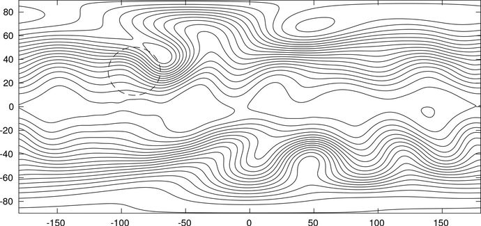
Göran Starius. 2020. On the use of reduced grids in conjunction with the Equator-Pole grid system.
… mostly? §
Why “… mostly?” Notice that among the neatly laid out hexagonal grid, the corners of each icosahedron face are each one triangle short of a hexagon. That’s because the icosahedron’s vertices started out 5-triangle and stay that way after subdivision. They form 12 pentagons in this grid, then persist after any additional subdivision. So, to a geospatial data scientist, a hexagonal global grid like H3 is “trillions of hexagons and 12 pentagons.”
On the other hand, game developers might want to show a 100% hexagonally-gridded globe map without such artifacts required by the laws of mathematics. For them, binning cells and showing data accurately are of lesser concern, let alone defeating topology, so they have devised tricks to hide the pentagons.
So how? And why? §
With that survey of cartography over, I’ll summarize:
- The big Part I if is dead, replaced by a more nuanced objective that accepts unavoidable distortion: to distribute the distortion where it hurts the least for some specific definition of hurts.
- In my case, I’ve decided somewhat arbitrarily that I want the triangles to have equal area. To that end, none of the methods I’ve tried so far are close to optimal. But, direct slerp handily beats recursive midpoint, which is most definitely not the gold standard I thought it was (with more subdivision, it doesn’t even eventually converge to equal area!).
- I’ve also confirmed that an icosahedron is the best root solid for subdivision, a process as simple as putting eyes on the fugliness of octaspheres and tetraspheres, but also bolstered by research into geospatial geodesic grids.
I started out optimizing a seemingly-academic graphics problem nobody had, then built prototypes that yielded big surprises, leading me to dig way deeper into the geometry, and finally came across a field of cutting-edge geospatial computing research with higher stakes and much deeper rabbit holes than even the course I had charted for myself. Now I have to take stock and figure out where to go from here.
The asymmetry in direct slerp suggests there is still structure left to optimize. Because the “direct slerp” approach seems promising, I see a few likely paths for the technical optimization. But a better strategy, honestly, is to spend serious time studying projection/carto literature and software practice before reinventing the trapezoidal rule.
As for the technical optimization, I have some ideas and I’ll compare them based on how promising they seem for idiosyncratic naming:
- Move from pairwise edge-wise slerp constructions toward a weighted spherical average over three vertices, a generalized version of slerp (which is itself a weighted average over two points on the sphere). This could easily generate a grid of new vertices while operating in a barycentric coordinate system to directly translate from the planar triangle to the spherical triangle. I could name it direct direct slerp, or direct-er slerp, or slerp-er-er…
- We want dihedral symmetry, so we make the algorithm itself dihedral symmetric: run direct slerp three times, once towards each edge of the triangle, then average the results. Or instead of producing rows of vertices along two edges towards the third, produce them “outside-in”: from the edges towards the centroid, and where each new vertex is repeated with 120º symmetry. Definitely a few flavors to try here, and the di-f’ing-rect-hedral nomenclature is wide open for appellation shenanigans.
- We want optimal triangles and we have quantified optimization metrics. We also have so. many. numerical. optimization. algorithms. Maybe we don’t need a principled approach at all: just throw the problem at a black-box optimizer with a beefy GPU and see what oozes out. I don’t love the distinctive naming potential of this approach, but maybe we can work “creativity of handle” into the optimization error function to also delegate that to John Compute.
- Similar to above, but maybe we don’t need a black-box optimizer and instead some opinionated gradient descent approach that exploits the structure of the problem. Maybe the resulting field of vertices is the result of some iterative process that gradually relaxes the vertices into a more optimal configuration, like a physics simulation of repelling particles or something¤¤. This could be a rich mine of dank sobriquets, but I smell some damp. See, gradient is denoted by nabla. Y’know,
See you in another sixteen years.
Appendix: to Mercator apologists §
In case you expected a take here about Mercator projection as a product and perpetuator of colonialism, please remind yourself that someone writing about distortion inside of icosahedral map tiles has hot takes that are way more pedantic than that dead horse. My main matter with Mercator—the man, the method, and the map—is that the ostensibly revolutionary utility in navigation supposedly enabled by Mercator’s 1569 map and its projection is vastly overstated, and its rate of adoption mythologized.
At its core, the technological advance underpinning Mercator apologists is that it allowed sailors to chart a course of constant heading between two ports by drawing a straight line between them on either (depending on how hard they apologize) the or a Mercator map.
The geometry behind that is the best kind of correct and intuitive to us GPS-brain Mt. Stupid campers. But it’s actually not useful for navigation in the era before longitude, whose measurement is a surprisingly recent technological development. Specifically, without the ability to measure longitude accurately, the special use of the Mercator to easily chart constant-heading (rhumb) line courses ran into two issues***.
One, there existed no large-scale survey of magnetic declination with which to actually determine true heading from a compass measurement.
The other, I suppose more significantly, people who couldn’t measure longitude didn’t know where anything was, at least not with enough accuracy to make navigating by heading useful. Instead, courses were either mapped using Portolan charts (ever-shifting highly-connected undirected graphs of compass bearings & distance) or charted like driving directions: sail straight north or south to the destination’s latitude, then hang a lou-/rooie, and finally stay on that latitude until you hit the destination or get wrecked by the kraken. Keep in mind too, that there was no diesel option to sail against the wind. So even the use of a compass heading is not exactly straightforward with actual sailcraft courses†††.
And besides, where did Mercator get the data to construct his map? The same nautical charts that were already in use, of course. But, he ignored or didn’t know the distinction between latitude charts and Portolan charts, as well as mapmaking conventions such as a non-uniform scale in latitude to make the Isthmus of Suez look better‡‡‡. Granted, this was the best data available at the time, but it still left the Mercator 1569 map an academic novelty. The projection, whose parallel meridians saw it soon adopted by cartographers, didn’t see widespread use amongst mariners for centuries.
As for Web Mercator being simply an evolution of what users have come to expect, I think that’s likely begging the question. Obviously, squares in the world should remain square on screen and circles—even LHC-sized circles—should remain circles, so shape preservation is important. And “north-up” orientation is how we learned to read maps. But even if we didn’t defend Web Mercator just because it’s what we have, the apologism still embeds an assumption that a world map projection is needed at all for local mapping software.
When zoomed in at a city scale, the area in view is a lot smaller than “the globe.” As we covered here, smaller areas of a sphere are better approximations of flat surfaces. The tradeoffs made between different map projections don’t matter at this scale; just about any will do, so long as the software centers that projection’s sweet spot(s) in the view. And why not zoom out to a space view of the 3D globe? Flattening a globe distorts it, so… don’t. Indeed, this is the default behavior for Apple Maps and the underdocumented Globe View option for Google Maps§§§. Funnily enough, the supposed technical advantages of Web Mercator also come with drawbacks, as (for example) grumbled by this software engineer who designed and implemented Google Maps’s spherical mode.